JiT (Just Image Transformers)#
https://arxiv.org/pdf/2511.13720
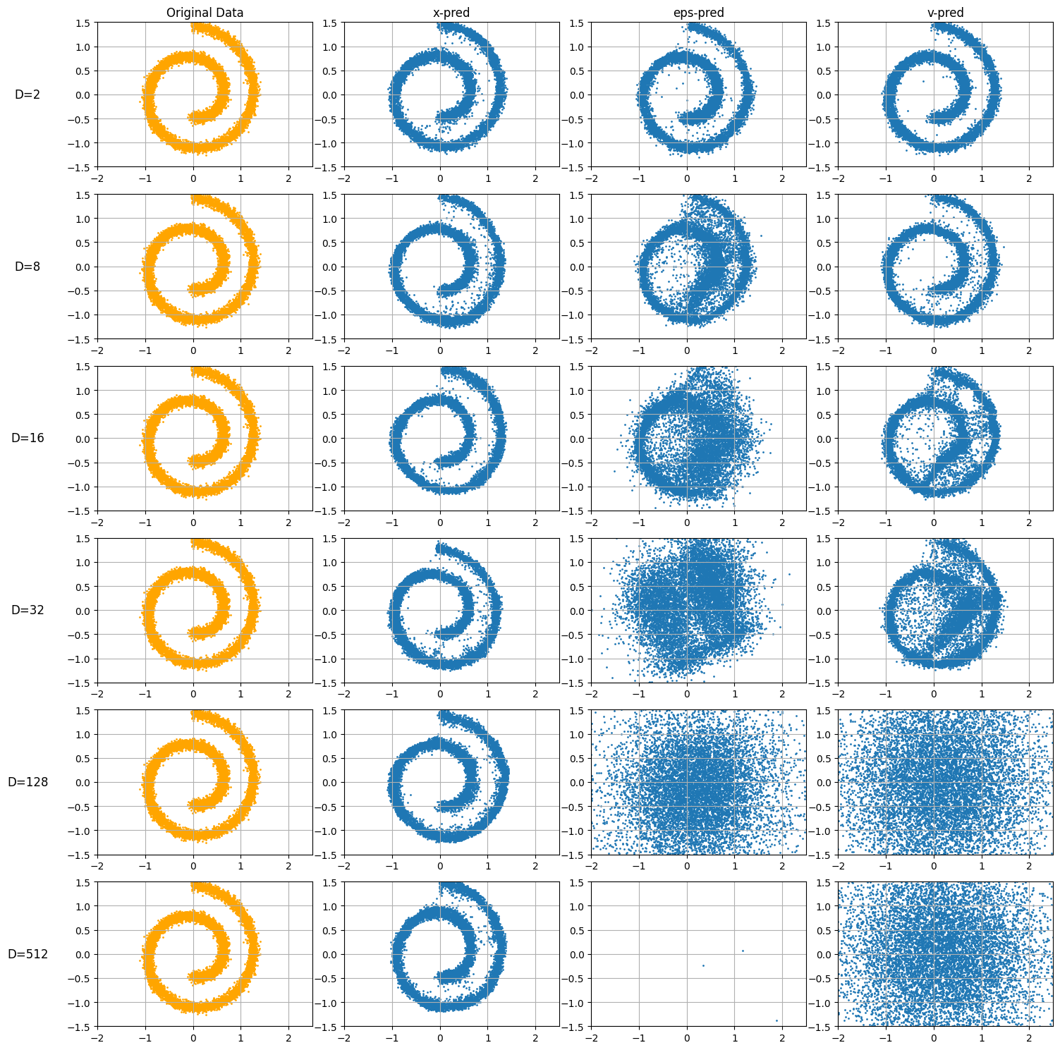
JiT argues x-prediction is often preferable because clean data \(x\) lies on a low-dimensional manifold (easier for networks to learn), while ε and v span high-dimensional space off-manifold.
During generation/sampling, transform the network output to the v-space (to solve the ODE \(\frac{dz_t}{dt} = v_\theta(z_t, t)\))
This notebook will implement the toy example from the paper using JAX, training a MLP to generate the SWISS roll embedded in a high AMBIENT dimension, to prove this point.
import jax
import jax.numpy as jnp
from jax import random, numpy as np, lax, vmap
import optax
import equinox as eqx
from tqdm import tqdm

import jax
import jax.numpy as jnp
from sklearn.datasets import make_swiss_roll, make_moons
N = 10000
def get_spiral_data(batch_size, noise=0.02):
data, _ = make_swiss_roll(batch_size, noise=noise)
data = data[:, [0, 2]] / 10.0
return jnp.array(data)
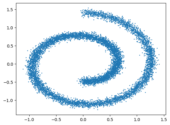
data = get_spiral_data(N,noise=.5)
import matplotlib.pyplot as plt
plt.scatter(x=data[:,0],y=data[:,1],s=1.0)
<matplotlib.collections.PathCollection at 0x7efdf0204e10>
class MLP(eqx.Module):
  layers: list

  def __init__(self,key,D):
    keys = jax.random.split(key, 6)
    hidden_dim = 256
    szs = [D+1] + 4*[hidden_dim] + [D]

    self.layers = []
    for i,(in_dim,out_dim,key) in enumerate(zip(szs[:-1],szs[1:],keys[1:])):
      layer = eqx.nn.Linear(in_dim,out_dim,key = key)
      self.layers.append(layer)

  def __call__(self,x,t):
    # Concatenate x (D) and t (scalar)
    x = jnp.concatenate([x, t], axis=-1)
    # (D+1)
    for layer in self.layers[:-1]:
      x = layer(x)
      x = jax.nn.relu(x)
    x = self.layers[-1](x)
    return x
V-Losses#
By parameterizing the network output as an \(x\)-prediction,\(v\)-prediction, or \(\epsilon\)-prediction, we can obtain the other two quantities with the two relevant equations in flow matching.
where \(x \sim p_{data}\) and \(\epsilon \sim \mathcal{N}(0, I)\).
For example, if we parameterize the network to predict \(x\), i.e \(x_\theta = \text{net}_\theta (z_t,t)\), the above two equations form consistency conditions that any triplet \(x_\theta, \epsilon_\theta, v_\theta\) must satisfy at each timestep.
By consistency conditions, we mean the other two variables (\(\epsilon_\theta\) and \(v_\theta\)) are completely determined by the constraints above.
by construction, \(x_\theta\) directly from the network.
forward-process consistency: whatever clean image \(x_\theta\) and noise \(\epsilon_\theta\) the model believes in, they must reproduce the actually observed \(z_t\) when interpolated
velocity-definition consistency: the predicted velocity is defined to be exactly \(x - \epsilon\).
We obtain \(v_\theta\) by rearranging the second equation and plugging into the third.
Then, we train with our v-loss as normal: $\(L_{v} = \mathbb{E}_{t, x, \epsilon} \left[ \| v_\theta - (x-\epsilon) \|^2 \right]\)$
This notebook focuses on the \(v\)-loss space for simplicity.
def x_pred_v_loss(model,x,z_t,t,eps):
  '''
  model: nn making x-prediction
  x: sampled from p_data
  pred: output of the network
  z_t: the interpolation between x and eps
  t: time step
  eps: noise
  '''
  v_target = x-eps
  x_pred = vmap(model)(z_t,t)
  v_theta = (x_pred - z_t)/(1-t).clip(.01,1-.01)
  return jnp.mean((v_target-v_theta)**2)

def v_pred_v_loss(model,x,z_t,t,eps):
  '''
  model: nn making v-prediction
  x: sampled from p_data
  pred: output of the network
  z_t: the interpolation between x and eps
  t: time step
  eps: noise
  '''
  v_target = x-eps
  v_pred = vmap(model)(z_t,t)
  return jnp.mean((v_target-v_pred)**2)

def eps_pred_v_loss(model,x,z_t,t,eps):
  '''
  model: nn making eps-prediction
  x: sampled from p_data
  pred: output of the network
  z_t: the interpolation between x and eps
  t: time step
  eps: noise
  '''
  v_target = x-eps
  eps_pred = vmap(model)(z_t,t)
  v_theta = (z_t - eps_pred) / t.clip(.05,1-.05)
  return jnp.mean((v_target-v_theta)**2)
Training Loop#
Slow Training Loop#
def logistic(x):
  return 1.0 / (1.0 + jnp.exp(-x))

def make_step(mlp,x,optim, opt_state,key,loss_fn):
  '''
  Compute loss and take gradient step on sampled data
  '''
  step_key, noise_key = random.split(key,2)
  t = random.uniform(step_key,shape=(cfg['batch_size'],1))
  # t = logistic(t)
  t=t.clip(.01,1-.01)
  # (B,1)
  eps = random.normal(noise_key,shape=x.shape)
  # (B, D)
  z_t = t * x + (1-t) * eps
  # (B, D)

  loss_value, grads = eqx.filter_value_and_grad(loss_fn)(mlp, x,z_t,t,eps)

  updates, opt_state = optim.update(
        grads, opt_state, eqx.filter(mlp, eqx.is_array)
    )
  mlp = eqx.apply_updates(mlp, updates)

  return mlp,opt_state,loss_value

def train_model(cfg, key, P, data, pred_type, loss_type = 'v_loss'):
  mlp = MLP(key,cfg['D'])
  optim = optax.adam(cfg['lr'])
  opt_state = optim.init(eqx.filter(mlp, eqx.is_array))

  if pred_type == 'x_prediction':
    loss_fn = x_pred_v_loss
  elif pred_type == 'v_prediction':
    loss_fn = v_pred_v_loss
  elif pred_type == 'eps_prediction':
    loss_fn = eps_pred_v_loss

  @eqx.filter_jit
  def step_fn(mlp, x, opt_state, key):
      return make_step(mlp, x, optim, opt_state, key, loss_fn)

  losses = []
  num_batches = data.shape[0] // cfg['batch_size']
  for step in tqdm(range(cfg['epochs'])):
    key, perm_key = random.split(key,2)
    perm = random.permutation(perm_key, data.shape[0])
    shuffled_data = data[perm]

    epoch_loss = 0
    for i in range(num_batches):
      key, train_key = random.split(key)
      x_hat = shuffled_data[i*cfg['batch_size'] : (i+1)*cfg['batch_size']]
      # (B,2)
      x = x_hat@P.T
      # (B,D)
      mlp, opt_state, train_loss = step_fn(mlp,x,opt_state,train_key)
      epoch_loss += train_loss
    losses.append(epoch_loss/num_batches)

  # print(f"Step={step} Loss={epoch_loss/num_batches}")
  # plt.plot(losses)
  # plt.show()

  return mlp
Fast Training Loop#
def logistic(x):
    return 1.0 / (1.0 + jnp.exp(-x))

def make_step_scanned(carry, batch_data, optim, static_loss_fn, P):
    mlp, opt_state, key = carry

    x_hat = batch_data

    # projection inside JIT so it's fused and fast
    x = x_hat @ P.T

    step_key, noise_key, next_key = random.split(key, 3)

    t = random.uniform(step_key, shape=(x.shape[0], 1))
    t = t.clip(.01, 1-.01)
    eps = random.normal(noise_key, shape=x.shape)
    z_t = t * x + (1-t) * eps

    loss_value, grads = eqx.filter_value_and_grad(static_loss_fn)(mlp, x, z_t, t, eps)

    updates, opt_state = optim.update(
        grads, opt_state, eqx.filter(mlp, eqx.is_array)
    )
    mlp = eqx.apply_updates(mlp, updates)

    return (mlp, opt_state, next_key), loss_value

def train_model(cfg, key, P, data, pred_type, loss_type='v_loss'):
    mlp = MLP(key, cfg['D'])
    optim = optax.adam(cfg['lr'])
    opt_state = optim.init(eqx.filter(mlp, eqx.is_array))

    if pred_type == 'x_prediction':
        loss_fn = x_pred_v_loss
    elif pred_type == 'v_prediction':
        loss_fn = v_pred_v_loss
    elif pred_type == 'eps_prediction':
        loss_fn = eps_pred_v_loss

    num_train_samples = data.shape[0]
    # drop the last incomplete batch to keep shapes uniform for scan
    num_batches = num_train_samples // cfg['batch_size']
    # truncate data to fit perfectly into batches
    data_truncated = data[:num_batches * cfg['batch_size']]

    def run_epoch(carrier, data_shuffled):
        # scan automatically iterates over the first dimension of data_shuffled
        # data_shuffled shape: (num_batches, batch_size, input_dim)

        final_carrier, losses = jax.lax.scan(
            lambda c, x: make_step_scanned(c, x, optim, loss_fn, P),
            carrier,
            data_shuffled
        )
        return final_carrier, jnp.mean(losses)

    # 3. JIT epoch loop
    @eqx.filter_jit
    def train_epoch_jit(mlp, opt_state, key, data_epoch):
        # reshape data to (num_batches, batch_size, features)
        data_reshaped = data_epoch.reshape(num_batches, cfg['batch_size'], -1)

        carrier = (mlp, opt_state, key)
        (mlp, opt_state, key), epoch_loss = run_epoch(carrier, data_reshaped)

        return mlp, opt_state, key, epoch_loss

    losses = []

    for step in tqdm(range(cfg['epochs'])):
        key, perm_key = random.split(key)

        perm = random.permutation(perm_key, data_truncated.shape[0])
        shuffled_data = data_truncated[perm]

        mlp, opt_state, key, epoch_loss = train_epoch_jit(mlp, opt_state, key, shuffled_data)

        losses.append(epoch_loss)

    return mlp
ODE Solvers#
# x_{t+h} = x_t + h * v_theta(x,t)
def x_euler_step(model_fn,z,t,dt):
  # z:  (num_samples, D)
  # t:  scalar
  t_vec = jnp.full((1,), t) # (1,)
  x_pred = vmap(model_fn,in_axes=(0,None))(z,t_vec)  # in_axes (0,None) indicates to parallelize over batch, and pass same t
  v_hat = (x_pred - z)/(1-t)
  return z + dt*v_hat,z

# x_{t+h} = x_t + h * v_theta(x,t)
def v_euler_step(model_fn,z,t,dt):
  # z:  (num_samples, D)
  # t:  (num_samples,)
  t_vec = jnp.full((1,), t)
  v_hat = vmap(model_fn,in_axes=(0,None))(z,t_vec)
  return z + dt*v_hat,z

# x_{t+h} = x_t + h * v_theta(x,t)
def eps_euler_step(model_fn,z,t,dt):
  # z:  (num_samples, D)
  # t:  scalar
  t_vec = jnp.full((1,), t) # (1,)
  eps_pred = vmap(model_fn,in_axes=(0,None))(z,t_vec)
  v_hat = (z-eps_pred)/(t)
  return z + dt*v_hat,z
Train and sample for each D#
from functools import partial
vpreds = []
xpreds = []
eps_preds = []
Ps = []

cfg = {
    'epochs': 2000,
    'batch_size': 1024,
    'lr': 1e-3,
    'D': 2
}

num_samples = 10000
num_steps = 100

key = jax.random.PRNGKey(42)
ts = jnp.linspace(.01,1.0-.01,num_steps)
dt = ts[1] - ts[0]  # Constant step size

d_keys = jax.random.split(key,6)
Ds = [2, 8, 16, 32, 128, 512]
for i in range(len(Ds)):
  d = Ds[i]
  cfg['D'] = d
  # Generate random projection
  A = random.normal(d_keys[i],(cfg['D'], 2))
  # P is a orthonormal projection matrix
  P, _ = jnp.linalg.qr(A)
  P = jnp.array(P)

  print(f"Training x-prediction for dimension {d}")
  mlp_x = train_model(cfg, d_keys[i], P, data, pred_type="x_prediction")
  print(f"Training eps-prediction for dimension {d}")
  mlp_eps = train_model(cfg, d_keys[i], P, data, pred_type="eps_prediction")
  print(f"Training v-prediction for dimension {d}")
  mlp_v = train_model(cfg, d_keys[i], P, data, pred_type="v_prediction")

  x0 = random.normal(d_keys[i],(num_samples,cfg['D']))
  # (num_samples, D)

  step_fn_x = partial(x_euler_step, mlp_x,dt=dt)
  step_fn_eps = partial(eps_euler_step, mlp_eps,dt=dt)
  step_fn_v = partial(v_euler_step, mlp_v,dt=dt)

  x1_xpred, history = lax.scan(step_fn_x,init=x0,xs=ts)
  x1_eps_pred, history = lax.scan(step_fn_eps,init=x0,xs=ts)
  x1_vpred, history = lax.scan(step_fn_v,init=x0,xs=ts)

  xpreds.append(x1_xpred)
  eps_preds.append(x1_eps_pred)
  vpreds.append(x1_vpred)
  Ps.append(P)
Training x-prediction for dimension 2
0%| | 0/2000 [00:00<?, ?it/s]
100%|██████████| 2000/2000 [00:09<00:00, 205.05it/s]
Training eps-prediction for dimension 2
100%|██████████| 2000/2000 [00:08<00:00, 225.81it/s]
Training v-prediction for dimension 2
100%|██████████| 2000/2000 [00:08<00:00, 230.21it/s]
Training x-prediction for dimension 8
100%|██████████| 2000/2000 [00:09<00:00, 220.56it/s]
Training eps-prediction for dimension 8
100%|██████████| 2000/2000 [00:08<00:00, 226.11it/s]
Training v-prediction for dimension 8
100%|██████████| 2000/2000 [00:08<00:00, 229.24it/s]
Training x-prediction for dimension 16
100%|██████████| 2000/2000 [00:09<00:00, 212.42it/s]
Training eps-prediction for dimension 16
100%|██████████| 2000/2000 [00:08<00:00, 223.75it/s]
Training v-prediction for dimension 16
100%|██████████| 2000/2000 [00:08<00:00, 229.10it/s]
Training x-prediction for dimension 32
100%|██████████| 2000/2000 [00:08<00:00, 222.27it/s]
Training eps-prediction for dimension 32
100%|██████████| 2000/2000 [00:08<00:00, 229.27it/s]
Training v-prediction for dimension 32
100%|██████████| 2000/2000 [00:08<00:00, 233.81it/s]
Training x-prediction for dimension 128
100%|██████████| 2000/2000 [00:09<00:00, 204.59it/s]
Training eps-prediction for dimension 128
100%|██████████| 2000/2000 [00:09<00:00, 216.27it/s]
Training v-prediction for dimension 128
100%|██████████| 2000/2000 [00:09<00:00, 217.10it/s]
Training x-prediction for dimension 512
100%|██████████| 2000/2000 [00:11<00:00, 167.41it/s]
Training eps-prediction for dimension 512
100%|██████████| 2000/2000 [00:11<00:00, 171.95it/s]
Training v-prediction for dimension 512
100%|██████████| 2000/2000 [00:12<00:00, 166.19it/s]
Visualize#
fig, axes = plt.subplots(6, 4, figsize=(15, 15))
column_titles = ["Original Data", "x-pred", "eps-pred", "v-pred"]
for i in range(4):
  axes[0, i].set_title(column_titles[i])

for i in range(6):
  P = Ps[i]
  axes[i,0].scatter(data[:,0],data[:,1],s=1.0,c='orange')
  axes[i,0].set_ylabel(f"D={Ds[i]}", rotation=0, fontsize=12, labelpad=40, va='center')
  for j in range(4):
    axes[i,j].set_xlim(-2, 2.5)
    axes[i,j].set_ylim(-1.5, 1.5)
    axes[i,j].grid(True)

  x_hat_xpred = xpreds[i] @ P
  axes[i,1].scatter(x_hat_xpred[:,0],x_hat_xpred[:,1],s=1.0)
  x_hat_eps_pred = eps_preds[i] @ P
  axes[i,2].scatter(x_hat_eps_pred[:,0],x_hat_eps_pred[:,1],s=1.0)
  x_hat_vpred = vpreds[i] @ P
  axes[i,3].scatter(x_hat_vpred[:,0],x_hat_vpred[:,1],s=1.0)

fig.tight_layout()