import jax
import jax.numpy as jnp
from jax import random, numpy as np, lax, vmap
import optax

key = jax.random.PRNGKey(42)

Score Matching

This post will serve two functions: to explain what a score function is, and to demonstrate the basics of JAX.

A score function is the gradient of the log probability density function with respect to the input.

\[ S(x) = \nabla_x \log p(x) \]

Surprisingly, Hyvärinen et al. showed we can estimate this function without knowing the density function \(p(x)\) itself.

How do we estimate it?

If we had the density, we could minimize the L2 loss between the true score function and our estimated score function \(s_\theta(x)\) parameterized by \(\theta\):

\[\begin{split} \begin{align} L(\theta) &= \frac{1}{2} \mathbb E_{x\sim p}\bigg[ || s_\theta(x) - \nabla_x \log p(x) ||^2_2 \bigg] \\ \end{align} \end{split}\]

However, since we don’t have the density , we can do some clever manipulation to remove this dependency. $\( \begin{align*} L(\theta) &= \frac{1}{2} \int p(x) || s_\theta(x) ||^2 dx - \underbrace{\int p(x) s_\theta(x)^T \nabla_x \log p(x) dx}_{\text{expanding log term}} + \frac{1}{2} \int p(x) || \nabla_x \log p(x) ||^2 dx \\ & \qquad \qquad \qquad \qquad \qquad \qquad \qquad \qquad \Large\downarrow \\ &= \frac{1}{2} \int p(x) || s_\theta(x) ||^2 dx - \underbrace{\left( \int \cancel {p(x)} s_\theta(x)^T \frac{\nabla_x p(x)}{\cancel{p(x)}}dx\right)}_{\text{multi-dimensional IBP where u= } s_\theta(x)^T, dv = \nabla_x p(x) dx} +\frac{1}{2} \int p(x) || \nabla_x \log p(x) ||^2 dx \\ & \qquad \qquad \qquad \qquad \qquad \qquad \qquad \qquad \Large\downarrow \\ &= \frac{1}{2} \int p(x) || s_\theta(x) ||^2 dx - \left( \underbrace{s_\theta(x)^T p(x)\big|_{-\infty}^{\infty}}_{\text{boundary term}} - \int p(x) (\nabla_x \cdot s_\theta(x))dx\right)+ \underbrace{\frac{1}{2} \int p(x) || \nabla_x \log p(x) ||^2 dx}_{\text{constant w.r.t. } \theta} \\ &= \mathbb E_{x\sim p}\bigg[ \frac{1}{2} || s_\theta(x) ||^2 + Tr(\nabla_x s_\theta(x)) \bigg] + C \end{align*} \)$

Great, now we can approximate the expectation with samples from \(p(x)\) and minimize the loss using gradient descent! JAX is new to me, so the below is mainly about JAX, and future posts will be about the difficulties of score matching, which motivates diffusion models.

Create Data

# create a mixture of gaussians
def create_dataset(mus,sigmas,ws,n_samples=20000):
  keys = jax.random.split(key, len(mus) + 1)
  samples = []
  for mu, sigma, w, current_key in zip(mus, sigmas, ws, keys):
    num_samples = int(n_samples * w)
    samples.append(random.normal(current_key, shape=(num_samples,)) * sigma + mu)
  return jnp.concatenate(samples)

mus = [-2,2]
sigmas = [1,1]
ws = [.5,.5]
dataset = create_dataset(mus,sigmas,ws)

# plot
import matplotlib.pyplot as plt
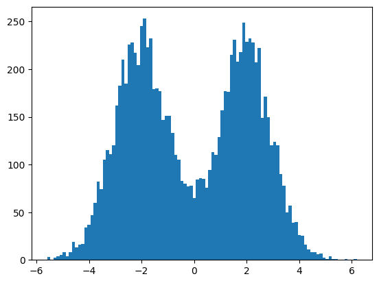
plt.hist(dataset,bins=100)
plt.show()

We have a created a simple 1D equal mixture of Gaussians.

The interesting part of this is to note is that JAX uses pure functions, which means

1. For the same input, the function will always return the same output

2. The function has no side effects (it doesn’t modify any external state)

In this case, this poses a problem for random generation, since if we call random.normal with the same key for each Gaussian, we will get the same samples every time. Instead, we have to explicitly get \(\mu_1,...\) different keys by ‘jax.random.split’ because that is how many Gaussians we have in our mixture.

Create MLP

szs = [1,1024]
out_dim = 1
szs = szs + [out_dim]
def create_mlp(szs):
  keys = random.split(key,len(szs))
  params = []
  for in_sz, out_sz, cur_key in zip(szs[:-1],szs[1:],keys):
    w_key, b_key = random.split(cur_key,2)
    w = random.normal(w_key,(in_sz,out_sz))
    b = random.normal(b_key,(out_sz,))
    params.append((w,b))
  return params

params = create_mlp(szs)

def relu(x):
  return jnp.maximum(0, x)

def forward(params, x):
  """
  params: list of weights and biases
  x: a single example of shape [feature_sz, ]
  """
  out = x
  for w,b in params[:-1]:
    out = jnp.dot(out,w) + b
    out = jax.nn.softplus(out)

  # output layer
  final_w, final_b = params[-1]
  out = jnp.dot(out,final_w) + final_b
  return out

Similarly to creating a random key for each Gaussian, we have to create a random key with “random.split” for each layer of the MLP, so each layer is not randomized to the same values.

Loss Function and Gradient Calculation

There are two ways to calculate gradients from a mini-batch. We can calculate the gradient for each example in the batch, and then average the gradients. Alternatively, we can average the loss over the batch, and then take the gradient of that average loss. Both give the same gradients as the gradient of the average loss is the same as the average of the gradients. However, the former is more efficient, since it only requires one backward pass through the network, instead of one backward pass per example in the batch.

Per-datapoint gradients (the inefficient way)

def score_matching_loss(params, x):
  """
  model: list of weights and biases
  x: shape [feature_sz,]
  """
  s_x = lambda x : forward(params, x)
  trace_term = jnp.trace(jax.jacfwd(s_x)(x))
  norm_term = .5 * jnp.sum(s_x(x))**2
  return trace_term + norm_term

model_to_loss_and_grad = jax.value_and_grad(score_matching_loss,argnums=0)

@jax.jit
def make_step(params, opt_state, batch):
  losses, grads = jax.vmap(model_to_loss_and_grad,in_axes=(None,0))(params, batch)
  # inaxes indicates to parallelize over the batch and use the same params for each

  loss = jnp.mean(losses)
  print(params)
  grad = jax.tree_util.tree_map(lambda g: jnp.mean(g, axis=0), grads)

  updates, opt_state = optimizer.update(grad, opt_state)
  params = optax.apply_updates(params, updates)
  return loss, params, opt_state

vmap will vectorize the provided function over the specified axis. Since I just learned about vmap, my first thought was to create a loss function that would work for one example, and then vectorize over the batch. In this case, we want to vectorize over the batch axis (the 0th axis) of the input data, while keeping the model parameters the same for each datapoint in the batch (hence in_axes=(None, 0)).

But, we also want the gradient, not just the loss. The value_and_grad function computes both the value of the loss function and its gradient with respect to the model parameters. argnums indicates what input variable(s) of a function will be differentiated wrt. In our case, we explictly indicates that we want to differentiate with respect to the model parameters with argnums=0. If you pass in a tuple, then you will get a tuple of gradients. By using vmap, we apply this function to each example in the batch, resulting in a list of losses and gradients.

However, this is inefficient, since it requires one backward pass per example in the batch. Interestingly, this also exposed me to another JAX concept, Pytrees, when trying to compute the average gradient. Pytrees are nested structures of python containers (like lists, tuples, and dictionaries), called branches, that can hold data (like arrays or scalars) at the leaves. In our case, the model parameters \([(w1,b1), (w2,b2), \dots]\) are a list of tuples, so the outer list is a branch, and each tuple is a nested branch, with the weights and biases as leaves.

Pytrees give us the flexibility to do handy operations like vmap,grad,etc on complex data structures, like params. However, this means we cannot just call jnp.mean(grads) because the gradients will also be a nested list of tuples, an undefined operation. More specifically, the data at the leaves of the gradients will have an extra batch dimension, since we calculated the gradient for each example in the batch. We extract the mean over this batch dimension for each leaf in the nested structure by using jax.tree_util.tree_map, which walks though the entire PyTree, applying a function we specificy to each leaf. This is exactly lambda g: jnp.mean(g, axis=0).

Per-batch gradient (the efficient way)

def score_matching_loss(params, x):
  """
  model: list of weights and biases
  x: shape [feature_sz,]
  """
  s_x = lambda x : forward(params, x)
  trace_term = jnp.trace(jax.jacfwd(s_x)(x))
  norm_term = .5 * jnp.sum(s_x(x))**2
  return trace_term + norm_term

def batch_loss(params, batch):
  # inaxes indicates to parallelize loss calculation over the batch and use the same params for each
  return jnp.mean(jax.vmap(score_matching_loss,in_axes=(None,0))(params, batch))

@jax.jit
def make_step(params, opt_state, batch):
  loss, grad = jax.value_and_grad(batch_loss)(params, batch)

  updates, opt_state = optimizer.update(grad, opt_state)
  params = optax.apply_updates(params, updates)
  return loss, params, opt_state

Now, that we’ve seen the inefficient approach, we can see that the efficient approach is much simpler. We just need to create a batch_loss function that averages the loss over the batch by using vmap to vectorize the score_matching_loss function over the batch axis of the input data (again using in_axes=(None, 0)). Then, we can use value_and_grad on this batch_loss function to get the loss and gradient in one backward pass.

It is worth noting grad is still a PyTree, but since we only calculated one gradient for the entire batch, there is no extra batch dimension to average over. This means its PyTree structure \([\text{(grad_w1,grad_b1),(grad_w2,grad_b2)}]\) is the same as params, so we can directly use it in optax.apply_updates, which requires the gradient to have the same structure as the parameters.

Main Training Loop

learning_rate = 5e-3
epochs = 500
batch_size = 2048
optimizer = optax.adam(learning_rate)
opt_state = optimizer.init(params)

model_key, train_key = random.split(key,2)
num_batches = len(dataset) // batch_size
losses = []
for epoch in range(epochs):
  mb_losses = []
  for i in range(num_batches):
    train_key, choice_key, step_key = random.split(train_key,3)
    indices = random.choice(choice_key,len(dataset),shape=(batch_size,),replace=False)
    batch = dataset[indices]

    loss, params, opt_state = make_step(params, opt_state, batch)
    mb_losses.append(loss)
  loss = jnp.mean(jnp.array(mb_losses))
  losses.append(loss)
  print(f'Epoch: {epoch}, Loss: {loss}')

Epoch: 0, Loss: 3177.72265625
Epoch: 1, Loss: 211.29458618164062
Epoch: 2, Loss: 291.1797790527344
Epoch: 3, Loss: 121.80747985839844
Epoch: 4, Loss: 24.00171661376953
Epoch: 5, Loss: 30.262611389160156
Epoch: 6, Loss: 5.925556182861328
Epoch: 7, Loss: 5.7019453048706055
Epoch: 8, Loss: 1.3145476579666138
Epoch: 9, Loss: 1.019349217414856
Epoch: 10, Loss: 0.1265537291765213
Epoch: 11, Loss: -0.02911228872835636
Epoch: 12, Loss: -0.1976195126771927
Epoch: 13, Loss: -0.22964665293693542
Epoch: 14, Loss: -0.2720133364200592
Epoch: 15, Loss: -0.2750064432621002
Epoch: 16, Loss: -0.29703372716903687
Epoch: 17, Loss: -0.28125348687171936
Epoch: 18, Loss: -0.29429832100868225
Epoch: 19, Loss: -0.2701902389526367
Epoch: 20, Loss: -0.27173498272895813
Epoch: 21, Loss: -0.2711723744869232
Epoch: 22, Loss: -0.2721530497074127
Epoch: 23, Loss: -0.2969388961791992
Epoch: 24, Loss: -0.2988685071468353
Epoch: 25, Loss: -0.29066142439842224
Epoch: 26, Loss: -0.2817121148109436
Epoch: 27, Loss: -0.2844347059726715
Epoch: 28, Loss: -0.28856489062309265
Epoch: 29, Loss: -0.2969137728214264
Epoch: 30, Loss: -0.3180720806121826
Epoch: 31, Loss: -0.30118444561958313
Epoch: 32, Loss: -0.28756192326545715
Epoch: 33, Loss: -0.31076207756996155
Epoch: 34, Loss: -0.30098584294319153
Epoch: 35, Loss: -0.29123762249946594
Epoch: 36, Loss: -0.3091075122356415
Epoch: 37, Loss: -0.3032325208187103
Epoch: 38, Loss: -0.2887538969516754
Epoch: 39, Loss: -0.3214336037635803
Epoch: 40, Loss: -0.30178454518318176
Epoch: 41, Loss: -0.298456609249115
Epoch: 42, Loss: -0.30445295572280884
Epoch: 43, Loss: -0.30441051721572876
Epoch: 44, Loss: -0.29912418127059937
Epoch: 45, Loss: -0.3079603612422943
Epoch: 46, Loss: -0.2995204031467438
Epoch: 47, Loss: -0.3060549795627594
Epoch: 48, Loss: -0.30162450671195984
Epoch: 49, Loss: -0.29701903462409973
Epoch: 50, Loss: -0.31048744916915894
Epoch: 51, Loss: -0.29925018548965454
Epoch: 52, Loss: -0.30645203590393066
Epoch: 53, Loss: -0.3096816837787628
Epoch: 54, Loss: -0.30543604493141174
Epoch: 55, Loss: -0.3058070242404938
Epoch: 56, Loss: -0.31420421600341797
Epoch: 57, Loss: -0.30258265137672424
Epoch: 58, Loss: -0.3136073350906372
Epoch: 59, Loss: -0.3181304931640625
Epoch: 60, Loss: -0.30897778272628784
Epoch: 61, Loss: -0.31562143564224243
Epoch: 62, Loss: -0.30938032269477844
Epoch: 63, Loss: -0.31281524896621704
Epoch: 64, Loss: -0.30774441361427307
Epoch: 65, Loss: -0.3203660249710083
Epoch: 66, Loss: -0.31329283118247986
Epoch: 67, Loss: -0.30242711305618286
Epoch: 68, Loss: -0.30780887603759766
Epoch: 69, Loss: -0.3164137899875641
Epoch: 70, Loss: -0.31017234921455383
Epoch: 71, Loss: -0.31467998027801514
Epoch: 72, Loss: -0.3079206645488739
Epoch: 73, Loss: -0.31449487805366516
Epoch: 74, Loss: -0.32100871205329895
Epoch: 75, Loss: -0.31847044825553894
Epoch: 76, Loss: -0.3061079978942871
Epoch: 77, Loss: -0.3123840391635895
Epoch: 78, Loss: -0.3002050220966339
Epoch: 79, Loss: -0.3163602650165558
Epoch: 80, Loss: -0.3114754557609558
Epoch: 81, Loss: -0.32115790247917175
Epoch: 82, Loss: -0.31743595004081726
Epoch: 83, Loss: -0.30366796255111694
Epoch: 84, Loss: -0.3098119795322418
Epoch: 85, Loss: -0.32037147879600525
Epoch: 86, Loss: -0.33052849769592285
Epoch: 87, Loss: -0.32200106978416443
Epoch: 88, Loss: -0.3250916600227356
Epoch: 89, Loss: -0.3086307644844055
Epoch: 90, Loss: -0.3061180114746094
Epoch: 91, Loss: -0.32849881052970886
Epoch: 92, Loss: -0.3129817247390747
Epoch: 93, Loss: -0.32367029786109924
Epoch: 94, Loss: -0.3151518404483795
Epoch: 95, Loss: -0.3102587163448334
Epoch: 96, Loss: -0.3252103328704834
Epoch: 97, Loss: -0.31333696842193604
Epoch: 98, Loss: -0.3218823969364166
Epoch: 99, Loss: -0.3189854025840759
Epoch: 100, Loss: -0.31202051043510437
Epoch: 101, Loss: -0.3098639249801636
Epoch: 102, Loss: -0.31216204166412354
Epoch: 103, Loss: -0.31543371081352234
Epoch: 104, Loss: -0.31458303332328796
Epoch: 105, Loss: -0.3113575577735901
Epoch: 106, Loss: -0.3071177005767822
Epoch: 107, Loss: -0.3020639717578888
Epoch: 108, Loss: -0.32499200105667114
Epoch: 109, Loss: -0.32231125235557556
Epoch: 110, Loss: -0.31534335017204285
Epoch: 111, Loss: -0.3113420009613037
Epoch: 112, Loss: -0.3171471059322357
Epoch: 113, Loss: -0.3139441907405853
Epoch: 114, Loss: -0.3288818895816803
Epoch: 115, Loss: -0.3178001344203949
Epoch: 116, Loss: -0.3170461058616638
Epoch: 117, Loss: -0.3172086179256439
Epoch: 118, Loss: -0.3236183822154999
Epoch: 119, Loss: -0.3208400011062622
Epoch: 120, Loss: -0.31135204434394836
Epoch: 121, Loss: -0.33417126536369324
Epoch: 122, Loss: -0.32795974612236023
Epoch: 123, Loss: -0.3117727041244507
Epoch: 124, Loss: -0.31418269872665405
Epoch: 125, Loss: -0.32812610268592834
Epoch: 126, Loss: -0.32573166489601135
Epoch: 127, Loss: -0.3115195333957672
Epoch: 128, Loss: -0.30545756220817566
Epoch: 129, Loss: -0.33160141110420227
Epoch: 130, Loss: -0.32108280062675476
Epoch: 131, Loss: -0.32622233033180237
Epoch: 132, Loss: -0.32019707560539246
Epoch: 133, Loss: -0.3215491771697998
Epoch: 134, Loss: -0.3349599540233612
Epoch: 135, Loss: -0.31583699584007263
Epoch: 136, Loss: -0.3141043186187744
Epoch: 137, Loss: -0.3238193392753601
Epoch: 138, Loss: -0.32112133502960205
Epoch: 139, Loss: -0.3241303861141205
Epoch: 140, Loss: -0.33931514620780945
Epoch: 141, Loss: -0.3198238015174866
Epoch: 142, Loss: -0.3320575952529907
Epoch: 143, Loss: -0.3220049738883972
Epoch: 144, Loss: -0.3236880600452423
Epoch: 145, Loss: -0.32601556181907654
Epoch: 146, Loss: -0.324209988117218
Epoch: 147, Loss: -0.33412256836891174
Epoch: 148, Loss: -0.3187941312789917
Epoch: 149, Loss: -0.32448312640190125
Epoch: 150, Loss: -0.3303185999393463
Epoch: 151, Loss: -0.3217243254184723
Epoch: 152, Loss: -0.3305867612361908
Epoch: 153, Loss: -0.3249867856502533
Epoch: 154, Loss: -0.3161279261112213
Epoch: 155, Loss: -0.32218122482299805
Epoch: 156, Loss: -0.3396650552749634
Epoch: 157, Loss: -0.31851115822792053
Epoch: 158, Loss: -0.3264182507991791
Epoch: 159, Loss: -0.3169742524623871
Epoch: 160, Loss: -0.3262702524662018
Epoch: 161, Loss: -0.3191661238670349
Epoch: 162, Loss: -0.32343047857284546
Epoch: 163, Loss: -0.32263505458831787
Epoch: 164, Loss: -0.30212393403053284
Epoch: 165, Loss: -0.33245742321014404
Epoch: 166, Loss: -0.32291826605796814
Epoch: 167, Loss: -0.3167029023170471
Epoch: 168, Loss: -0.3277667462825775
Epoch: 169, Loss: -0.3315131664276123
Epoch: 170, Loss: -0.33467498421669006
Epoch: 171, Loss: -0.3161507248878479
Epoch: 172, Loss: -0.33029448986053467
Epoch: 173, Loss: -0.3252844214439392
Epoch: 174, Loss: -0.31624531745910645
Epoch: 175, Loss: -0.3276044726371765
Epoch: 176, Loss: -0.3306345045566559
Epoch: 177, Loss: -0.3229348957538605
Epoch: 178, Loss: -0.3335762321949005
Epoch: 179, Loss: -0.32679954171180725
Epoch: 180, Loss: -0.33444610238075256
Epoch: 181, Loss: -0.31914663314819336
Epoch: 182, Loss: -0.33106595277786255
Epoch: 183, Loss: -0.3349761664867401
Epoch: 184, Loss: -0.3277984857559204
Epoch: 185, Loss: -0.3328416347503662
Epoch: 186, Loss: -0.3268076479434967
Epoch: 187, Loss: -0.3437609374523163
Epoch: 188, Loss: -0.33881065249443054
Epoch: 189, Loss: -0.34122011065483093
Epoch: 190, Loss: -0.3255924880504608
Epoch: 191, Loss: -0.33618032932281494
Epoch: 192, Loss: -0.32692840695381165
Epoch: 193, Loss: -0.3314919173717499
Epoch: 194, Loss: -0.32505515217781067
Epoch: 195, Loss: -0.3368656039237976
Epoch: 196, Loss: -0.33425191044807434
Epoch: 197, Loss: -0.33588603138923645
Epoch: 198, Loss: -0.32152456045150757
Epoch: 199, Loss: -0.3269830644130707
Epoch: 200, Loss: -0.3264737129211426
Epoch: 201, Loss: -0.3334690034389496
Epoch: 202, Loss: -0.3328602612018585
Epoch: 203, Loss: -0.32196730375289917
Epoch: 204, Loss: -0.3386955261230469
Epoch: 205, Loss: -0.32729941606521606
Epoch: 206, Loss: -0.3212118148803711
Epoch: 207, Loss: -0.3343047797679901
Epoch: 208, Loss: -0.33308401703834534
Epoch: 209, Loss: -0.3305472433567047
Epoch: 210, Loss: -0.34678542613983154
Epoch: 211, Loss: -0.33937591314315796
Epoch: 212, Loss: -0.32894426584243774
Epoch: 213, Loss: -0.3477964997291565
Epoch: 214, Loss: -0.32526424527168274
Epoch: 215, Loss: -0.3352905809879303
Epoch: 216, Loss: -0.33156073093414307
Epoch: 217, Loss: -0.33635541796684265
Epoch: 218, Loss: -0.33586475253105164
Epoch: 219, Loss: -0.33257928490638733
Epoch: 220, Loss: -0.3288152515888214
Epoch: 221, Loss: -0.3354189991950989
Epoch: 222, Loss: -0.3268955945968628
Epoch: 223, Loss: -0.33241841197013855
Epoch: 224, Loss: -0.31985336542129517
Epoch: 225, Loss: -0.3367719054222107
Epoch: 226, Loss: -0.3268299102783203
Epoch: 227, Loss: -0.3392293155193329
Epoch: 228, Loss: -0.33603301644325256
Epoch: 229, Loss: -0.33400899171829224
Epoch: 230, Loss: -0.3324045240879059
Epoch: 231, Loss: -0.3360896408557892
Epoch: 232, Loss: -0.3339335024356842
Epoch: 233, Loss: -0.336657851934433
Epoch: 234, Loss: -0.3277508318424225
Epoch: 235, Loss: -0.34014183282852173
Epoch: 236, Loss: -0.3356679379940033
Epoch: 237, Loss: -0.33505362272262573
Epoch: 238, Loss: -0.3361826241016388
Epoch: 239, Loss: -0.3298197388648987
Epoch: 240, Loss: -0.3405243456363678
Epoch: 241, Loss: -0.3352375626564026
Epoch: 242, Loss: -0.3460729420185089
Epoch: 243, Loss: -0.3335484564304352
Epoch: 244, Loss: -0.3357781767845154
Epoch: 245, Loss: -0.33686891198158264
Epoch: 246, Loss: -0.33702927827835083
Epoch: 247, Loss: -0.3425520360469818
Epoch: 248, Loss: -0.3361717760562897
Epoch: 249, Loss: -0.32421690225601196
Epoch: 250, Loss: -0.34203413128852844
Epoch: 251, Loss: -0.34860387444496155
Epoch: 252, Loss: -0.3363941013813019
Epoch: 253, Loss: -0.33872056007385254
Epoch: 254, Loss: -0.332205206155777
Epoch: 255, Loss: -0.3389209806919098
Epoch: 256, Loss: -0.347114622592926
Epoch: 257, Loss: -0.3298276364803314
Epoch: 258, Loss: -0.3366364538669586
Epoch: 259, Loss: -0.348641037940979
Epoch: 260, Loss: -0.3240099549293518
Epoch: 261, Loss: -0.33765825629234314
Epoch: 262, Loss: -0.3391417860984802
Epoch: 263, Loss: -0.3304923176765442
Epoch: 264, Loss: -0.3398232161998749
Epoch: 265, Loss: -0.33632537722587585
Epoch: 266, Loss: -0.33222976326942444
Epoch: 267, Loss: -0.3380044400691986
Epoch: 268, Loss: -0.34740760922431946
Epoch: 269, Loss: -0.3398689925670624
Epoch: 270, Loss: -0.3453853130340576
Epoch: 271, Loss: -0.35012948513031006
Epoch: 272, Loss: -0.34219351410865784
Epoch: 273, Loss: -0.3491763174533844
Epoch: 274, Loss: -0.347562700510025
Epoch: 275, Loss: -0.3441435992717743
Epoch: 276, Loss: -0.3437556326389313
Epoch: 277, Loss: -0.340741366147995
Epoch: 278, Loss: -0.32561418414115906
Epoch: 279, Loss: -0.3365088999271393
Epoch: 280, Loss: -0.3456626236438751
Epoch: 281, Loss: -0.34356650710105896
Epoch: 282, Loss: -0.33889010548591614
Epoch: 283, Loss: -0.346342533826828
Epoch: 284, Loss: -0.3495731055736542
Epoch: 285, Loss: -0.35330334305763245
Epoch: 286, Loss: -0.34286966919898987
Epoch: 287, Loss: -0.3397924602031708
Epoch: 288, Loss: -0.3370493948459625
Epoch: 289, Loss: -0.3452112674713135
Epoch: 290, Loss: -0.34011220932006836
Epoch: 291, Loss: -0.3388855457305908
Epoch: 292, Loss: -0.34292376041412354
Epoch: 293, Loss: -0.34415504336357117
Epoch: 294, Loss: -0.34101709723472595
Epoch: 295, Loss: -0.3461126387119293
Epoch: 296, Loss: -0.3296727240085602
Epoch: 297, Loss: -0.3328024446964264
Epoch: 298, Loss: -0.3453448414802551
Epoch: 299, Loss: -0.3393959701061249
Epoch: 300, Loss: -0.34527868032455444
Epoch: 301, Loss: -0.334123432636261
Epoch: 302, Loss: -0.3397952616214752
Epoch: 303, Loss: -0.3391432762145996
Epoch: 304, Loss: -0.33681467175483704
Epoch: 305, Loss: -0.334816575050354
Epoch: 306, Loss: -0.3436006009578705
Epoch: 307, Loss: -0.3393253684043884
Epoch: 308, Loss: -0.34751400351524353
Epoch: 309, Loss: -0.3384149968624115
Epoch: 310, Loss: -0.3365301191806793
Epoch: 311, Loss: -0.33778706192970276
Epoch: 312, Loss: -0.3473767340183258
Epoch: 313, Loss: -0.3275875151157379
Epoch: 314, Loss: -0.33872324228286743
Epoch: 315, Loss: -0.3426142930984497
Epoch: 316, Loss: -0.3399725556373596
Epoch: 317, Loss: -0.34657812118530273
Epoch: 318, Loss: -0.3498551547527313
Epoch: 319, Loss: -0.340972363948822
Epoch: 320, Loss: -0.344287246465683
Epoch: 321, Loss: -0.34128546714782715
Epoch: 322, Loss: -0.3366098403930664
Epoch: 323, Loss: -0.3465432822704315
Epoch: 324, Loss: -0.3330747187137604
Epoch: 325, Loss: -0.35269781947135925
Epoch: 326, Loss: -0.34619268774986267
Epoch: 327, Loss: -0.34349608421325684
Epoch: 328, Loss: -0.347246378660202
Epoch: 329, Loss: -0.3528262674808502
Epoch: 330, Loss: -0.3320874571800232
Epoch: 331, Loss: -0.3413523733615875
Epoch: 332, Loss: -0.34765902161598206
Epoch: 333, Loss: -0.3496429920196533
Epoch: 334, Loss: -0.3413459360599518
Epoch: 335, Loss: -0.3319089114665985
Epoch: 336, Loss: -0.34907418489456177
Epoch: 337, Loss: -0.33845797181129456
Epoch: 338, Loss: -0.359964519739151
Epoch: 339, Loss: -0.34324488043785095
Epoch: 340, Loss: -0.3386978507041931
Epoch: 341, Loss: -0.34068241715431213
Epoch: 342, Loss: -0.3373476266860962
Epoch: 343, Loss: -0.3393406867980957
Epoch: 344, Loss: -0.3445023000240326
Epoch: 345, Loss: -0.34806400537490845
Epoch: 346, Loss: -0.34868767857551575
Epoch: 347, Loss: -0.3344227373600006
Epoch: 348, Loss: -0.335480660200119
Epoch: 349, Loss: -0.34421172738075256
Epoch: 350, Loss: -0.34987831115722656
Epoch: 351, Loss: -0.33089661598205566
Epoch: 352, Loss: -0.352789968252182
Epoch: 353, Loss: -0.3556446135044098
Epoch: 354, Loss: -0.34163275361061096
Epoch: 355, Loss: -0.34081971645355225
Epoch: 356, Loss: -0.346191942691803
Epoch: 357, Loss: -0.34468138217926025
Epoch: 358, Loss: -0.3534628450870514
Epoch: 359, Loss: -0.3463248312473297
Epoch: 360, Loss: -0.3415718376636505
Epoch: 361, Loss: -0.3402690589427948
Epoch: 362, Loss: -0.3419363796710968
Epoch: 363, Loss: -0.34677854180336
Epoch: 364, Loss: -0.338248074054718
Epoch: 365, Loss: -0.33955156803131104
Epoch: 366, Loss: -0.33202409744262695
Epoch: 367, Loss: -0.33643439412117004
Epoch: 368, Loss: -0.352140873670578
Epoch: 369, Loss: -0.35400906205177307
Epoch: 370, Loss: -0.3473832905292511
Epoch: 371, Loss: -0.32232382893562317
Epoch: 372, Loss: -0.32775476574897766
Epoch: 373, Loss: -0.34747710824012756
Epoch: 374, Loss: -0.3556682765483856
Epoch: 375, Loss: -0.35378608107566833
Epoch: 376, Loss: -0.3431250751018524
Epoch: 377, Loss: -0.34136343002319336
Epoch: 378, Loss: -0.34537041187286377
Epoch: 379, Loss: -0.3340968191623688
Epoch: 380, Loss: -0.343686580657959
Epoch: 381, Loss: -0.33998599648475647
Epoch: 382, Loss: -0.34239986538887024
Epoch: 383, Loss: -0.345205694437027
Epoch: 384, Loss: -0.34902137517929077
Epoch: 385, Loss: -0.33864378929138184
Epoch: 386, Loss: -0.34211546182632446
Epoch: 387, Loss: -0.3454718589782715
Epoch: 388, Loss: -0.34057486057281494
Epoch: 389, Loss: -0.34762972593307495
Epoch: 390, Loss: -0.35815107822418213
Epoch: 391, Loss: -0.34662169218063354
Epoch: 392, Loss: -0.3479554057121277
Epoch: 393, Loss: -0.34871307015419006
Epoch: 394, Loss: -0.33807173371315
Epoch: 395, Loss: -0.34808260202407837
Epoch: 396, Loss: -0.359452486038208
Epoch: 397, Loss: -0.33895233273506165
Epoch: 398, Loss: -0.34852638840675354
Epoch: 399, Loss: -0.34318217635154724
Epoch: 400, Loss: -0.32991790771484375
Epoch: 401, Loss: -0.3421079218387604
Epoch: 402, Loss: -0.34824085235595703
Epoch: 403, Loss: -0.3638869524002075
Epoch: 404, Loss: -0.34719768166542053
Epoch: 405, Loss: -0.349038302898407
Epoch: 406, Loss: -0.34504589438438416
Epoch: 407, Loss: -0.33732885122299194
Epoch: 408, Loss: -0.3454367518424988
Epoch: 409, Loss: -0.34569743275642395
Epoch: 410, Loss: -0.3454970121383667
Epoch: 411, Loss: -0.3399253189563751
Epoch: 412, Loss: -0.34654703736305237
Epoch: 413, Loss: -0.3447209894657135
Epoch: 414, Loss: -0.3481089472770691
Epoch: 415, Loss: -0.3414822816848755
Epoch: 416, Loss: -0.34379085898399353
Epoch: 417, Loss: -0.3419129550457001
Epoch: 418, Loss: -0.34846892952919006
Epoch: 419, Loss: -0.34170734882354736
Epoch: 420, Loss: -0.34240543842315674
Epoch: 421, Loss: -0.34352535009384155
Epoch: 422, Loss: -0.3373108506202698
Epoch: 423, Loss: -0.3357256352901459
Epoch: 424, Loss: -0.3380989134311676
Epoch: 425, Loss: -0.3502248525619507
Epoch: 426, Loss: -0.3458860516548157
Epoch: 427, Loss: -0.3426451086997986
Epoch: 428, Loss: -0.351467102766037
Epoch: 429, Loss: -0.3372788429260254
Epoch: 430, Loss: -0.34883585572242737
Epoch: 431, Loss: -0.3404478430747986
Epoch: 432, Loss: -0.3422659933567047
Epoch: 433, Loss: -0.3524221181869507
Epoch: 434, Loss: -0.3188188374042511
Epoch: 435, Loss: -0.34961262345314026
Epoch: 436, Loss: -0.3489070236682892
Epoch: 437, Loss: -0.3430608808994293
Epoch: 438, Loss: -0.35301193594932556
Epoch: 439, Loss: -0.3535463809967041
Epoch: 440, Loss: -0.3403187096118927
Epoch: 441, Loss: -0.3481631875038147
Epoch: 442, Loss: -0.35248374938964844
Epoch: 443, Loss: -0.35897889733314514
Epoch: 444, Loss: -0.35104456543922424
Epoch: 445, Loss: -0.35718783736228943
Epoch: 446, Loss: -0.3485780954360962
Epoch: 447, Loss: -0.33928436040878296
Epoch: 448, Loss: -0.3490864336490631
Epoch: 449, Loss: -0.33863702416419983
Epoch: 450, Loss: -0.3456023931503296
Epoch: 451, Loss: -0.34526491165161133
Epoch: 452, Loss: -0.3336217403411865
Epoch: 453, Loss: -0.34954676032066345
Epoch: 454, Loss: -0.3501238226890564
Epoch: 455, Loss: -0.3470989763736725
Epoch: 456, Loss: -0.3553963303565979
Epoch: 457, Loss: -0.35347384214401245
Epoch: 458, Loss: -0.3452093303203583
Epoch: 459, Loss: -0.3467203378677368
Epoch: 460, Loss: -0.33708539605140686
Epoch: 461, Loss: -0.3381357192993164
Epoch: 462, Loss: -0.34883809089660645
Epoch: 463, Loss: -0.3497549593448639
Epoch: 464, Loss: -0.3523820638656616
Epoch: 465, Loss: -0.34470391273498535
Epoch: 466, Loss: -0.3494519889354706
Epoch: 467, Loss: -0.34090951085090637
Epoch: 468, Loss: -0.3561747968196869
Epoch: 469, Loss: -0.3405098617076874
Epoch: 470, Loss: -0.3600464165210724
Epoch: 471, Loss: -0.34648963809013367
Epoch: 472, Loss: -0.33618590235710144
Epoch: 473, Loss: -0.33608824014663696
Epoch: 474, Loss: -0.3490085303783417
Epoch: 475, Loss: -0.33597859740257263
Epoch: 476, Loss: -0.3452760577201843
Epoch: 477, Loss: -0.3327758014202118
Epoch: 478, Loss: -0.3325687050819397
Epoch: 479, Loss: -0.3495647609233856
Epoch: 480, Loss: -0.3458164632320404
Epoch: 481, Loss: -0.3439997434616089
Epoch: 482, Loss: -0.3575357496738434
Epoch: 483, Loss: -0.3563772141933441
Epoch: 484, Loss: -0.35372626781463623
Epoch: 485, Loss: -0.33759409189224243
Epoch: 486, Loss: -0.36110129952430725
Epoch: 487, Loss: -0.34212517738342285
Epoch: 488, Loss: -0.35226139426231384
Epoch: 489, Loss: -0.33935150504112244
Epoch: 490, Loss: -0.3511958718299866
Epoch: 491, Loss: -0.3367750644683838
Epoch: 492, Loss: -0.3214203119277954
Epoch: 493, Loss: -0.3197283148765564
Epoch: 494, Loss: -0.34198129177093506
Epoch: 495, Loss: -0.34282493591308594
Epoch: 496, Loss: -0.35249224305152893
Epoch: 497, Loss: -0.34718599915504456
Epoch: 498, Loss: -0.3458236753940582
Epoch: 499, Loss: -0.3433145582675934

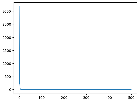
The only interesting part of the training loop is how we create the mini-batches. Again, since JAX uses pure functions, we have to explicitly split the random key at each step to get a new key for generating random indices for the mini-batch.

# plot loss
import matplotlib.pyplot as plt
plt.plot(losses)
plt.show()

True vs Expected Score

from jax import grad
from jax.scipy.stats import norm # Use JAX's SciPy stats for compatibility
import matplotlib.pyplot as plt


def mixture_norm_pdf(x, mus, sigmas, ws):
    mus = jnp.array(mus)
    sigmas = jnp.array(sigmas)
    ws = jnp.array(ws)

    pdf_values = ws * norm.pdf(x, loc=mus, scale=sigmas)

    return jnp.sum(pdf_values)

xs = jnp.arange(-4,4,.01)

# Calculate the true score function (gradient of log PDF)
def mixture_norm_log_pdf(x, mus, sigmas, ws):
    return jnp.log(mixture_norm_pdf(x, mus, sigmas, ws))

# Use jacfwd for scalar function and vmap for batching
true_score = vmap(jax.jacfwd(mixture_norm_log_pdf,argnums=0), in_axes=(0, None, None, None))

We know the true density function of our mixture of Gaussians, so we can calculate the true score function by taking the gradient of the log density function. First, we calculate the log PDF of the mixture of Gaussians, and then we use jax.jacfwd to take the gradient of this scalar function. Since we want to calculate the score function for multiple values of x, we use vmap to vectorize this gradient function over the input x values.

plt.plot(xs,true_score(xs, mus, sigmas, ws),label='true score')
plt.plot(xs,vmap(forward,in_axes=(None,0))(params,xs).squeeze(-1),label='learned score')

plt.legend()
plt.show()

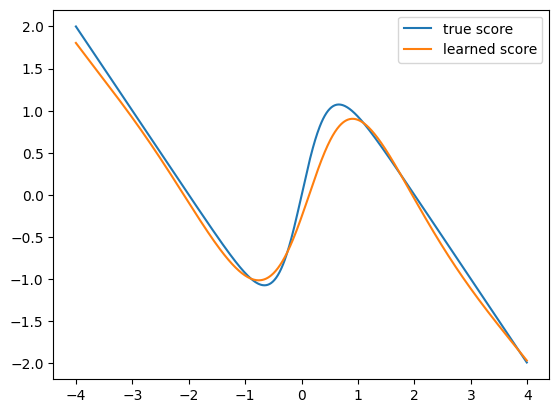
Great news! Our learned score function matches the true score function pretty well on this 1d toy dataset. We will see how this falls apart in our next blog post with high dimensional data.

Sampling with Langevin Dynamics

The scores tell us the direction of increasing likelihood, but that following this from some initial \(x_0\) will result in deterministic sampling. As a result, we follow the ‘noisy’ scores. This is called Langevin dynamics. When run for long enough with small enough steps, \(x_t \sim p(x)\).

\[ x_{t+1} = x_t + \alpha_t \nabla_x \log p(x_t) + \sqrt{2\alpha} z_t, \quad z_t \sim \mathcal N(0, I) \]

Since we don’t have the true score function, we will use our learned score function instead.

\[ x_{t+1} = x_t + \alpha_t s_\theta(x_t) + \sqrt{2\alpha} z_t, \quad z_t \sim \mathcal N(0, I) \]

alpha = 1e-2
n_particles = 10000
n_samples = 1000

def f(prev,key):
  epsilon = random.normal(key,shape=prev.shape)
  return prev + alpha*forward(params,prev)[0][0] + np.sqrt(2 * alpha)*epsilon, prev

def g(x,key):
  keys = random.split(key,n_samples)
  # in jax, functions must be pure, for the same key, random.normal must always return the same number
  # so we create an array of n_samples keys so that each step of langevin sampling, we get a new epsilon
  res, history = lax.scan(f,init=x,xs=keys)
  return res, history


xs = random.uniform(key,shape=(n_particles,))
keys = random.split(key,n_particles)
res, history = vmap(g)(xs,keys)

lax.scan is a handy function that allows us to carry state through a loop. In our case, we want to carry the current position of the particles through the Langevin dynamics steps. The f function is one step of Langevin dynamics. The g function runs n_samples steps of Langevin dynamics for one particle, using lax.scan to carry the state through the steps. lax.scan() takes three arguments: the function to apply at each step, the initial state init, and the sequence of inputs xs (data each timestep we want to reference) as we iterate. We can write f(carry,x)->(carry,y), where carry is the state we want to carry through the loop, x is the input at the current step, and y is the output at the current step.

In our case, lax.scan() will call f, n_samples times, passing the output of one step of Langevin dynamics as the input to the next call (the carry). The xs argument is an array of keys, one for each step, so that we can get a new random epsilon at each step. The init argument is the initial position of the particle. It returns the final position of the particle and the history of positions.

Since we want to run this for multiple particles, we use vmap to vectorize the g function over different initial positions.

The only wrinkle is that we need a new random key for each step of Langevin dynamics to get distinct epsilon for a particle over time and that this epsilon is distinct across particles as well. The latter is fulfilled by creating n_particles keys, feeding this into g, which creates n_samples child keys (number of Langevin steps) in f for each particle, fulfilling the former requirement.

That is why vmap(g) is called over the particles and keys.

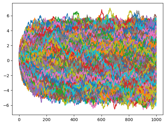
Visualize Evolution

# plot history of each evolution (second dim)
import matplotlib.pyplot as plt
for i in range(history.shape[0]):
  plt.plot(history[i,:,])
plt.show()

Visualize Samples

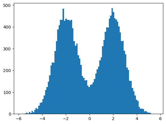
# plot final samples
import matplotlib.pyplot as plt
plt.hist(res[:],bins=100)
plt.show()